Bulk Good Laboratory Plant (BGLP)
This BGLP environment can be installed via:
import mlpro.rl.pool.envs.bglp
3rd Party Dependency
NumPy
Overview
The BGLP illustrates a smart production system with high flexibility and distributed control to transport bulk raw materials. One of the advantages of this laboratory test belt is the modularity in design, as depicted schematically below:
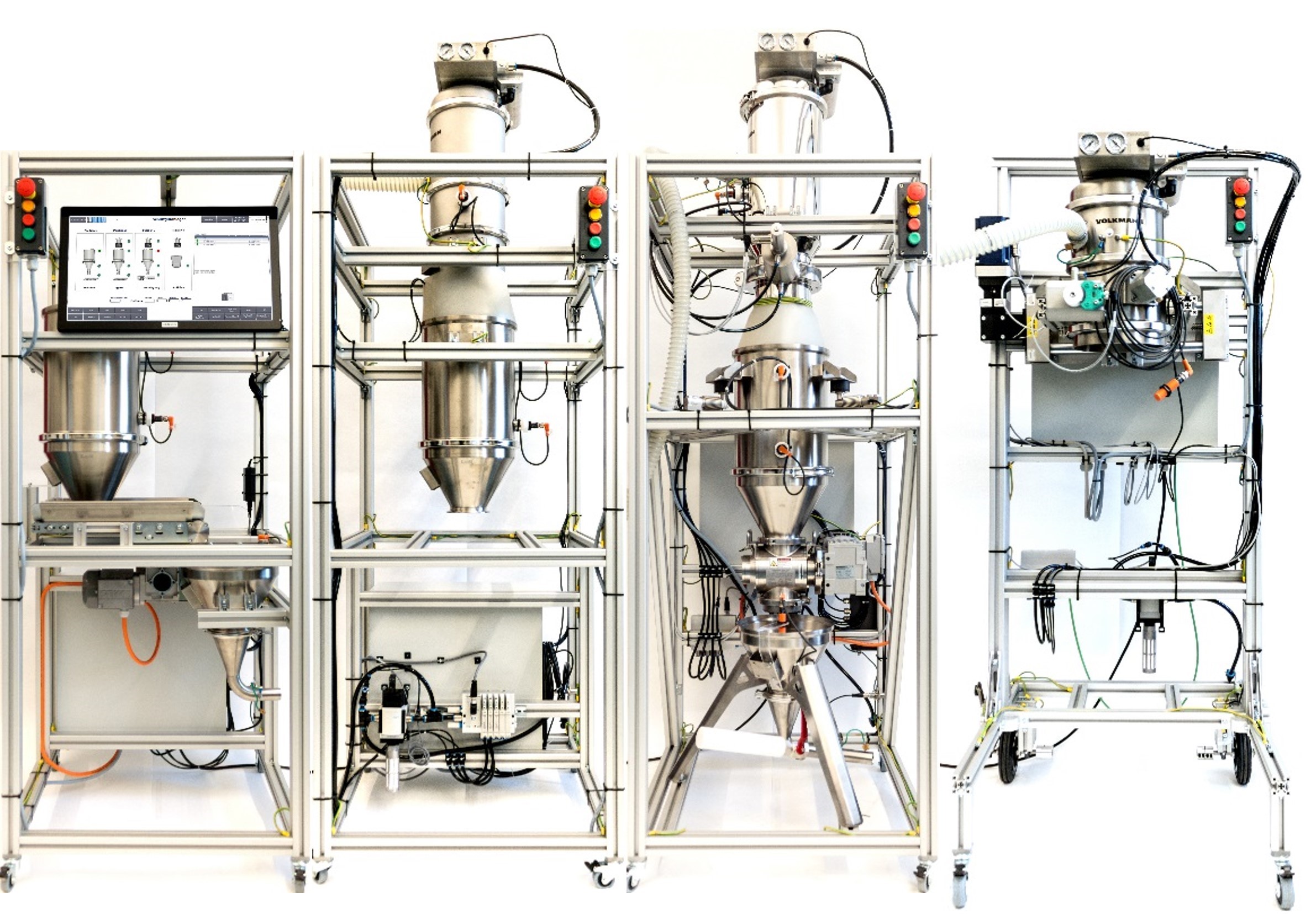
The BGLP consists of four modules, which are loading, storing, weighing, and filling stations respectively, and has conveying and dosing units as integral parts of the system. The interface between the modules is assembled via a mini hopper placed in the prior module. Then, the next module is fed by a vacuum pump, which operates in a discontinuous manner, before the goods are temporarily stored in a silo of the next module. The filling station has no silo because the main purpose of the station is to occupy the transport containers.
We utilize dissimilar actuators in modules 1-3 to transport the goods from the silo to the mini hopper. Module 1 utilizes a belt conveyor, that operates between 0 and 1800 rpm. Module 2 uses a vibratory conveyor, which can be completely switched on and off. Lastly, Module 3 utilizes a rotary feeder, that operates between 0 and 1450 rpm.
In theRL context, we consider the BGLP as a multi-agent system, where each actuator of the system is pointed as an agent or a player. The states information for each agent is the fill level of the prior reservoir and the fill level of the next reservoir.
Note
In this simulation, we assume that the actuator in Module D has a constant flow, which automatically matches the production demand in L/s. This parameter can be defined while setting up the BGLP environment. Therefore, 5 actuators are involved in this simulation instead of 6 actuators.
General information
Parameter
Value
Agents
5
Native Source
MLPro
Action Space Dimension
[5,]
Action Space Base Set
Real numbers, except Agent 3 uses Integer
Action Space Boundaries
[0,1]
State Space Dimension
[6,]
State Space Base Set
Real numbers
State Space Boundaries
[0,1]
Reward Structure
Individual reward for each agent
Note
You can change the configurations of the BGLP simulation, for instance, production demand (L/s), production target for batch operation (L), learning rates for reward calculation, and production scenario (batch or continuous). Batch production scenario refers to a process to satisfy a specific order in a sequence, thus the production target in L must be set. Meanwhile, continuous production scenario refers to a process to control a constant flow within a horizon, thus the production target (L) is not necessary and the target is fulfilled the production demand (L/s). The detailed explanations are available in the API reference section, see here.
Action space
In this environment, we consider 5 actuators to be controlled. Thus, there are 5 agents and 5 joint actions because each agent requires an action. Every action is normalized within a range between 0 and 1, except for Agent 3. 0 means the minimum possible action and 1 means the maximum possible action. For Agent 3, the vibratory conveyor has a different character than other actuators, which mostly perform in a continuous manner. The vibratory conveyor can only be either fully switched-on or switched-off. Therefore the base set of action for Agent 3 is an integer (0/1). 0 means off and 1 means on.
Agent
Actuator
Station
Parameter
Boundaries
1
Conveyor Belt
A
rpm
450 … 1800
2
Vacuum Pump
B
on-duration (sec)
0 … 4.575
3
Vibratory Conveyor
B
on/off
0/1
4
Vacuum Pump
C
on-duration (sec)
0 … 9.5
5
Rotary Feeder
C
rpm
450 … 1450
State space
The state information in the BGLP is the fill levels of the reservoirs. Each agent is always placed in between two reservoirs, e.g. between a silo and a hopper or vice versa. Therefore, each agent has two state information, which is shared with their neighbours. Every state is normalized within a range between 0 and 1. 0 means the minimum fill-level and 1 means the maximum fill-level.
Agent
State No.
Element
Station
Boundaries
1
1
Silo
A
0 … 17.42 L
2
Hopper
A
0 … 9.1 L
2
1
2
Silo
B
0 … 17.42 L
3
1
2
Hopper
B
0 … 9.1 L
4
1
2
Silo
C
0 … 17.42 L
5
1
2
Hopper
C
0 … 9.1 L
Reward structure
The reward structure is implemented according to this paper. You can also find the source code of the reward structure, here. The given reward is an individual scalar reward for each agent. To be noted, this reward function is more suitable for a continuous production scenario.
If you would like to implement a customized reward function, you can follow these lines of codes:
class MyBGLP(BGLP):

    def calc_reward(self):

        # Each agent has an individual reward
        if self.reward_type == Reward.C_TYPE_EVERY_AGENT:
            for actnum in range(len(self.acts)):
                acts = self.acts[actnum]
                self.reward[actnum] = 0
            return self.reward[:]

        # Overall reward
        elif self.reward_type == Reward.C_TYPE_OVERALL:
            self.overall_reward = 0
            return self.overall_reward
Version structure
Version 1.4.4 : Enhanchement, debug, refactoring, adding batch production scenario in MLPro v. 0.0.0
Version 1.0.0 : Initial version release in MLPro v. 0.0.0
If you apply this environment in your research or work, please kindly cite the following related paper:
@article{Schwung2021,
 title={Decentralized learning of energy optimal production policies using PLC-informed reinforcement learning},
 author={Dorothea Schwung and Steve Yuwono and Andreas Schwung and Steven X. Ding},
 journal={Comput. Chem. Eng.},
 year={2021},
 volume={152},
 pages={107382},
 doi={10.1016/j.compchemeng.2021.107382}
 }